Real-Time Soft-Object Animation Using Free-Form Deformation

Geometry in today’s games tends to be static. It's common to see animated characters composed of a hierarchy of meshes moving relative to each other, but it's rare to see the animation of individual vertices within a mesh.

Animating hierarchies of meshes (the common method) is a fine way to portray an object's movement, but does little to portray character or situation. In fields other than computer graphics, animators traditionally have exaggerated parts of a character to convey expressions. With current animation techniques, such exaggeration isn't possible. An object generally remains the same shape throughout the game.

Deforming the vertices within a mesh (the rare method) is the domain of soft-object animation. Until recently, this process was simply too expensive to consider in real-time. Soft-object animation is becoming computationally affordable, however, and can greatly enhance your animation.

There are many situations where a technique for deforming meshes could be applied in games:

We’re going to examine one of the simpler forms of soft-object animation - Free-form Deformation, commonly known as FFD. The technique has been around for some time, and was first documented in a SIGGRAPH paper by Sederburg and Parry in 1986. Programs such as 3D Studio Max have supported FFD both as a modeling and animation technique for some time, but it is only recently that the technique has become practical in real-time game engines.

At its heart, FFD is the metamorphosis of an object from its originally modeled appearance - known as the object’s rest state - to its deformed state. This is accomplished by deforming the object’s coordinate system in the following three steps:

This procedure will result in an object deformed in so that it is "intuitively consistent" with how we deformed the coordinate system. The term "intuitively consistent" is very popular in research papers on these subjects, but in practice it means that the deformed object looks like you hoped it would look. This allows artists to have confidence when using the technique in games.

Objects and Coordinate Systems

Usually, a polygon mesh object's shape is defined by the coordinates of its vertices in its local coordinate system. The cornerstone of FFD is that the position of the object’s vertices is not modified directly. Instead, the object’s local coordinate system is modified, which changes the resulting position of the object’s vertices in world space.

It's common in graphics to refer to "an object being rotated" or "an object being scaled." However, when describing FFDs, it is more useful to think in terms of coordinate systems – "the object’s local coordinate system is rotated, so the object appears to rotate." Thinking of the object in terms of changes to its local coordinate system means that the object can be animated in virtually any way so long as you deform its coordinate system appropriately.

So FFD has the advantage of being a very general technique. A particular FFD-generated effect can be applied to any object with similar results. It's also not limited to a particular type of object – FFDs are equally applicable to polygonal models, Bezier curves, or any other object representation. This generality makes the technique ideal for use in game engines.

Operations such as rotating and scaling are easy coordinate-system-based transformations to perform. Deformation techniques are not. They apply exactly the same operation to every vertex in the object, and straight lines in the object before the operation are still straight afterwards. If we have a coordinate system which supports bending or stretching more readily, the object will follow suit.

To accomplish this we’re going to define a coordinate system with more freedom than our regular (X, Y, Z) axes. It’s going to be based upon Bezier volumes, which are an extension of Bezier curves and surfaces. Because of this, FFDs are dependent upon Bezier theory - but since most of this theory is becoming commonplace in game graphics, this shouldn’t be a problem.

It’s often useful to visualize a new technique in terms of things with which you are already familiar. For instance, you can consider a Bezier curve a generalization of a straight-line segment. In fact, it's mathematically correct to say that a straight-line segment is "a Bezier curve of degree one." Similarly, a Bezier surface is a generalization of a plane, and a Bezier volume is just a generalization of a normal cubic volume. The only two differences between all these surface forms and their straight counterpoints are that 1) the surface forms are curved and 2) the number of points necessary to define them is greater.

So there's not a lot to it, then - as Jim Blinn said, "We use complicated math all the time. Most everyday math is just a specific case of something more complex."

A Review of Bezier Curves

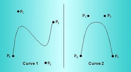
Fig. 1 shows two examples of Bezier curves. In fact, these are cubic Bezier curves – the kind that most computer graphics commonly use. I've labeled their control points P_0, P_1, P₂ and P₃, for each curve. The control points are a very important concept – they completely define the shape of the curve.

Figure 1

From an artist's perspective, the advantages of Bezier curves are clear. The curve is easy to specify via its control point because given just the control points it's easy to visualize how the resulting curve will look.

From the curves shown, it is easy to see the following:

Mathematical Definition of Bezier Curves

A curve is defined geometrically by its control points. We also need a mathematical formula to represent the shape of the curve, so that it can be reproduced on-screen. This section presents a brief derivation of the Bezier curve, leading to Eq. 4, which presents a single function for evaluating the kind of Bezier curve we will be using.

Higher degrees of equation allow more control points and therefore more complexly defined curves - all at the cost of greater computation time. Although it looks complicated, this representation is for a curve of arbitrary degree. In this article, we are going to deal with cubic curves, that it curves with n = 3. This kind of curve is defined by four control points and is particularly useful for defining FFDs.

A Bezier curve is defined by a parametric equation of the form:

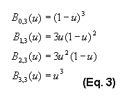
With the degree of curve fixed as 3, Eq. 2 can be expanded to produce four equations for

which are dependent only on the curve parameter u, as you can see in Eq. 3:

These functions are called the Bezier basis functions of degree three. You can use them to expand the sigma notation in Eq. 2. The result is a single function that we can use to evaluate the position on a cubic Bezier curve at any value of the parameter u:

We could draw the resulting curve by calculating the value of the function at a number of intervals and then connecting them with straight lines. Listing 1 shows code to evaluate Q(u) at any point on the curve.

Listing 1

CVector3D CEvaluator::EvalCurve(CURVECTRLPTS P, float u)
{

}

A Review of Bezier Surfaces

The notation of a curve extends easily to represent a surface. From the general form of the Bezier curve in Eq. 1, a parametric surface is a function of two parameters, termed u and v, as shown in Eq. 5:

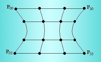
Since we have already established that we are interested only in cubic curves, we will only deal with cubic surfaces. A single Bezier surface is often called a patch, and Figure 2 shows a patch defined in two dimensions.

Figure 2

Again, it is clear that the control points define the shape of the patch. 16 control points define this one. Equation 6 represents the patch, and you will notice that it is similar in form to the Bezier curves in Eq. 2.

The array of control points P is extended from four vectors to a 4x4 array of vectors. The easiest way to think of a parametric surface is to imagine using the array's four rows to draw four horizontal curves, and then the array's four columns to draw four vertical curves. Together, these curves will produce a mesh of quadrilaterals.

Listing 2 shows code to evaluate the surface at any value of u and v in a similar manner to that in which Listing 1 would evaluate a curve:

Listing 2

CVector3D CEvaluator::EvalSurface(PATCHCTRLPTS P, float u, float v)

{

assert (P != NULL);

assert (u >= 0.0f && u <= 1.0f);

assert (v >= 0.0f && v <= 1.0f);

float BU[4], BV[4];

CVector3D Ret(0);

BU[0] = (1.0f - u) * (1.0f - u) * (1.0f - u);

BU[1] = 3.0f * u * (1 - u) * (1.0f - u);

BU[2] = 3.0f * u * u * (1.0f - u);

BU[3] = u * u * u;

BV[0] = (1.0f - v) * (1.0f - v) * (1.0f - v);

BV[1] = 3.0f * v * (1 - v) * (1.0f - v);

BV[2] = 3.0f * v * v * (1.0f - v);

BV[3] = v * v * v;

for (int i = 0; i < 4; i++) {

for (int j = 0; j < 4; j++) {

Ret += P[i][j] * (BU[i] * BV[j]);

}

}

return Ret;

}

Introducing Bezier Volumes

After defining Bezier curves and surfaces, the extension to volumes simply involves increasing the number of control points and adding another parameter to the Bezier equation. The array of control points P now contains 64 vectors in a 4x4x4 array, and the curve is defined in terms of three parameters as shown in Eq. 7:

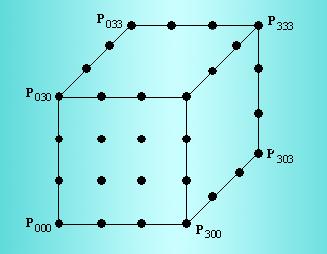
One of the most basic structures we can form the Bezier volume into is a cubic shape. To do this we set all the control points up to form a 4x4x4 regular coordinate grid. In this case the control points, drawn using 3D space, would look as shown in Fig. 3. Only the control points on the front face of the cube are drawn in full.

Figure 3

It's important to realize that a Bezier volume does not simply define a six-sided surface. It's a true volume, and you can freely alter the control points within it to produce a variety of volumes. As the control points are moved within the volume, the initially straight axes of the volume will deform to become Bezier curves.

Listing 3 shows code that will evaluate a position inside a Bezier volume for given u, v, and w parameter values.

Listing 3

CVector3D CEvaluator::EvalVolume(VOLUMECTRLPTS P, float u, float v, float w)

{

assert (P != NULL);

assert (u >= 0.0f && u <= 1.0f);

assert (v >= 0.0f && v <= 1.0f);

float BU[4], BV[4], BW[4];

CVector3D Ret(0);

BU[0] = (1.0f - u) * (1.0f - u) * (1.0f - u);

BU[1] = 3.0f * u * (1 - u) * (1.0f - u);

BU[2] = 3.0f * u * u * (1.0f - u);

BU[3] = u * u * u;

BV[0] = (1.0f - v) * (1.0f - v) * (1.0f - v);

BV[1] = 3.0f * v * (1 - v) * (1.0f - v);

BV[2] = 3.0f * v * v * (1.0f - v);

BV[3] = v * v * v;

BW[0] = (1.0f - w) * (1.0f - w) * (1.0f - w);

BW[1] = 3.0f * w * (1 - w) * (1.0f - w);

BW[2] = 3.0f * w * w * (1.0f - w);

BW[3] = w * w * w;

for (int i = 0; i < 4; i++) {

for (int j = 0; j < 4; j++) {

for (int k = 0; k < 4; k++) {

Ret += P[i][j] * (BU[i] * BV[j]);

}

}

return Ret;

}

The FFD Operation

For the purposes of this example, we’ll assume that an object is defined with only positive values for the (x, y, z) coordinates of its vertices. The bounding box of the object would then have its origin at (0, 0, 0) in object space and extend to (x_max, y_max, z_max). The resting state of the FFD block would match the bounding box of the object.

All Bezier curves, surfaces, and volumes are themselves examples of coordinate spaces. For a Bezier volume, a position with the volume is specified in terms of three coordinates, termed u, v, and w, and all assumed to vary between zero and one. Once an FFD block is defined around the object, each vertex in the object must be converted from its current (x, y, z) coordinate in the object to a (u, v, w) before deformation begins.

This parametric coordinate is known as the "lattice space" position of a vertex. Assuming the axes used for the FFD at rest are the X, Y, Z axes of the object’s local coordinate system, you can calculate this position by normalizing all coordinates in the object to line in the range 0-1:

After this, we deform the FFD block however we like. Update the values in the array of points P, and then plug the vertex’s lattice space coordinate into the Bezier volume equation. The returned vector will be the deformed position of the point.

After resultant position for every point is calculated, the model is drawn as usual. You can animate deformations by changing the positions of the control points every frame. An example of this is interpolating between one set of control points and another.

Extending the Control: Local Deformation

One disadvantage of using a single FFD block to control animation of an object is that you are applying global deformations. A deformation will alter the values of every vertex in the object to a greater or lesser extent. This gives the visual impression that the whole object is one jelly-like mass.

This is undesirable in many situations. For instance, we might be deforming a car as a result of a crash. If the car were to be hit at its front-right corner, we would want that corner of the car to crumple, but the rest of the car should remain unaffected.

We can apply changes more accurately to a particular part of the object by increasing the degree, and hence the number of control points, of the FFD. However, the changes applied are still global, and will still affect every point in the object, although to an increasingly small degree. The computational cost of the deformation is also greatly increased – remember that with an FFD block of degree n the inner loop is iterated n³ times per vertex.

The solution is to use more than one FFD block per object. In fact, there are no restrictions on the use of FFDs – they can even overlap within an object. We might define the car as being encased in four FFDs, one for each quarter of the car (as seen from above). Now during impact, if the first FFD block is modified, only the affected part of the car will change.

When joining FFDs the same continuity constraints apply as when joining Bezier curves or patches – that is, at a minimum, points which meet should be in the same position in space, and preferably should have some level of derivative continuity. This ensures that the object doesn’t develop any jagged edges or discontinuities during the deformation.

Bringing all the Theory Together

So far, we’ve talked about FFDs deforming the vertices of an object as if the object had to be polygonal. In practice, there is no reason for this to be the case. In fact, FFDs are particularly useful when combined with objects represented by Bezier patches. There are two reasons for this:

In practice, Bezier objects not only look better when used with FFDs, but they also require fewer calculations. If you’re already using Bezier objects in your game, there’s no reason not to implement FFDs, especially since they are so cheap.

Another way to reduce the number of calculations is to reduce the degree of the FFD block. While a cubic FFD requires 64 iterations of the function’s main loop per vertex to calculate the deformed positions, a quadratic FFD block, represented by a 3x3x3 array of control points, would only require 27 iterations. Linear FFDs, defined by a 2x2x2 grid of points can be used to quickly apply shear or taper to objects.

The sample application (deformation.zip) demonstrates the classic Utah Teapot, represented here as a Bezier-patch model, undergoing constant real-time deformation by a single FFD block. There is a readme.txt file describing the most interesting classes in the project to help you work out what’s going on in the code.

References

Watt, A. and Watt, M., Advanced animation and Rendering Techniques, Addison-Wesley, 1992.

Sederburg, T. W., Free-form Deformation of Solid Geometric Models, Proceedings from SIGGRAPH, 1985.

Bio

Alex Ferrier left Scotland at the tender age of 19 to go to work for Gremlin Interactive. There, he programmed for PlayStation titles such as Judge Dredd and Acuta Soccer 2 before moving on to PlayStation 3D engine programming with Actua Soccer 3. He's currently debating going back to university. He has lots of thoughts, but most of them are badly deformed. You can email him your straight ones at [email protected]