

Trending
Opinion: How will Project 2025 impact game developers?
The Heritage Foundation's manifesto for the possible next administration could do great harm to many, including large portions of the game development community.
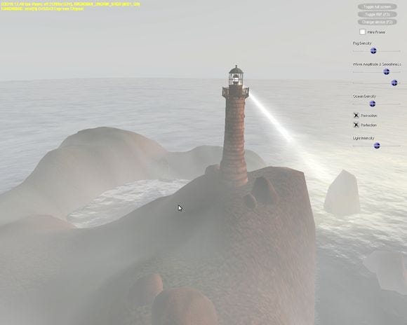
In a new Intel-sponsored feature from <a href="http://www.gamasutra.com/visualcomputing">the Visual Computing microsite</a>, a trio of Intel engineers showcase an experiment to create an ocean and complex fog effects using Direct3D 10 and Shader Model 4.0, complete with source code and executable demo.

[In this new Intel-sponsored feature from the Visual Computing microsite, a trio of Intel engineers showcase an experiment to create an ocean and complex fog effects using Direct3D 10 and Shader Model 4.0, complete with freely available source code and executable demo.]
The purpose of this project was to investigate how we could effectively render a realistic ocean scene on differing graphics solutions while trying to provide a current working class set of data to the graphics community.
Given the complexities involved with rendering an ocean as well as fog effects we chose to start by using a projected grid concept, because of its realistic qualities, as our baseline.
We then ported the original Direct3D 9 code to Direct3D 10 and also ported the additional effects we needed to convert to Shader Model 4.0. In doing so we took advantage of a great opportunity to learn about an interesting subject (the projected grid) while adding many more nuances to it.
In addition to determining how best to work with this complex system under a DirectX10 scenario, we also wanted to know what would be required to achieve reasonable frame rates on both low- and high-cost graphics solutions.
During this endeavor we learned much about how to offload certain computations to the CPU versus the GPU, as well as when and where those compute cycles would be the most beneficial, both on high-end and low-end graphics solutions. For example, on the CPU front, using the Intel Compiler (version 10.1), we were able to gain an easy 10+ fps on our CPU-side computations (to generate fog and approximate wave movement).
The basic concept behind the projected grid ocean is a regular discretized xz-plane that is displayed orthogonally to the viewer in world space. The vertices of this grid are then displaced using a height field. The height field is a product of two variables, which return the height value as specified by the following equation:
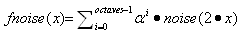
This method has proven very useful for generating a virtual large body of water.
The Perlin noise computation for generating the wave motion uses four textures of varying granularity called "octaves" to animate the grid in three dimensions. We chose this method to generate wave noise over other functions, such as Navier-Stokes, because it was less compute intensive on the CPU. The GPU-side Navier-Stokes implementation was not used, but it is worth further investigation. For reflections and refractions the algorithm uses derivations of Snell's function.
To further add realism to the scene we restricted the height of the camera on the y axis so that the illusion of ocean vastness could be maintained.
For a detailed description of this method, refer to Claes Johanson's Master Thesis.1
---
1 Johanson, Claes. "Real-time water rendering-introducing the projected grid concept." Master of Science thesis in computer graphics, March 2004. http://graphics.cs.lth.se/theses/projects/projgrid/, http://graphics.cs.lth.se/theses/projects/projgrid/projgrid-hq.pdf (PDF)
For the Perlin fog we decided to implement the processing on the CPU. To do this, we sampled points in the 3D texture space, separated by a stride associated with each octave-the longer the stride, the more heavily weighted the octave was in the total texture.
Each of these sample points was mapped to a pseudo randomly chosen gradient, using a permutation table full of normalized gradients from a given point and a hash function.1 The value of each pixel was then determined by the weight contributions of its surrounding gradient samples. All of these separate octaves were then summed to achieve a result that has smoothed organic noise on both a near and far perspective.
This result was successful; however, we wanted to achieve an even more smoothed effect and have only subtle noise visible. We then applied a simple Gaussian blur algorithm (also during preprocessing).

Our implementation blurred the pixels using factors supplied by Pascal's triangle constants, i.e., {(1), (1,1), (1,2,1), (1,3,3,1) . . . }, as weights and averaging those weighted sums (a type of convolution filter). We also took advantage of calculating blur independently in each axis direction to improve efficiency.2
At this point the result was much closer to the desired outcome; however, seams were visible at the edges of the texture because the Gaussian blur algorithm was sampling points beyond the texture's scope, so we used a mod operator to wrap the sampling space.
In the shader, we first calculated the fog coefficient f, which is a factor for the amount of light absorbed and scattered from a ray through fog volume.3 We calculated this value using the equation
f = e-(ρ*d*n)
where p=density, d=camera distance, and n=noise. We then used this coefficient to interpolate between the surface color Coriginal at any point and the fog color Cfog, using the equation This interpolation approximates the light absorption of a ray from any point to the camera4 at low CPU utilization cost.
Cfinal = Coriginal*f + Cfog*(1-f)
Finally, we applied animation to the fog by sampling the fog texture according to a linear function that progresses with time. This is a simple ray function with the slope set as a constant vector.
This method was successful, but it produced fog that appeared glued to the geometry surface rather than moving through the air. For this reason, we used a 3D texture for the blurry noise-when this texture is animated along a ray, the fog moves through world space rather than crawling along the surface's 2D texture coordinates.
This was successful from a bird's-eye perspective, but unconvincing at other perspectives. To adjust for this, we applied a quadratic falloff for our noise, dependent on the height of the fog; that is, it made the fog clearer at the height of the viewer to give the impression that clouds appeared above and below, rather than simply on all surfaces, with the equation
n = n*(ΔY2)/2 + 0.001
where n=noise and ∆Y=camera Y position - vertex Y position. As a result, we are able to mimic volumetric fog quite convincingly, although all fog is in fact projected onto the scene surfaces.
---
1 Johanson, Claes. "Real-time water rendering-introducing the projected grid concept." Master of Science thesis in computer graphics, March 2004.
http://graphics.cs.lth.se/theses/projects/projgrid/, http://graphics.cs.lth.se/theses/projects/projgrid/projgrid-hq.pdf (PDF)
2 Gustavson, Stefan, "Simplex Noise Demystified." Gabrielle Zachmann Personal Homepage, 22 Mar 2005. Linköping University, Sweden. 15 Jul 2008.
http://zach.in.tu-clausthal.de/teaching/cg2_08/literatur/simplexnoise.pdf (PDF)
3 Zdrojewska, Dorota, "Real time rendering of heterogeneous fog based on the graphics hardware acceleration." Central European Seminar on Computer Graphics for students. 3 Mar 2004.
Technical University of Szczecin. 10 Jul 2008. http://www.cescg.org/CESCG-2004/web/Zdrojewska-Dorota/
4 Waltz, Frederick M. and John W. V. Miller. "An efficient algorithm for Gaussian blur using finite-state machines." SPIE Conf. on Machine Vision Systems for Inspection and Metrology VII., 1 Nov. 1998.
ECE Department, Univ. of Michigan-Dearborn. 5 Aug. 2008. http://www-personal.engin.umd.umich.edu/~jwvm/ece581/21_GBlur.pdf (PDF)
The scene is lit entirely by two lights-one infinite (directional) light and one spotlight casting from the lighthouse. The infinite light is calculated simply by dot lighting with the light's direction and the vertex normals. The spotlight also uses dot lighting, but in addition takes into account a light frustum and falloff.
The stored information for the spotlight includes position, direction, and frustum. For surface lighting, we first determined whether a point lies within the spotlight frustum. Next we calculated falloff, and finally we applied the same dot lighting as used in the infinite light. For the first step, we found a vector from the vertex point to the camera, and then calculated the angle between that vector and the spotlight's direction vector, using a dot product rule and solving for the angle
V1 • V2 = | V1 | | V2| cos θ
where V1, V2 = vectors and θ = angle between. If the angle between the two vectors is within the frustum angle, we know that the point is illuminated by the spotlight. We then used this same angle to apply a gradual falloff for the spotlight. The difference between the calculated angle and the frustum angle determines how far away from the center of the frustum the point lies, so the falloff can be determined by the expression
| θfrustum / θ | - 1
where θ = angle between. As you can see, the expression is undefined at θ = 0 and less than or equal to 0 at θ > θfrustum. The undefined value computes to an infinitely large number during runtime, so we have exactly what we want-most intensity at the center of the frustum and no intensity at the edge. With this result, we used the HLSL saturate function to clamp these values between 0 and 1 and multiplied the spotlight intensity by this final number.

For the volumetric spotlight effect, we used the same frustum angle as before to construct a series of cones that amplifies the fog within the spotlight frustum. The cone vertices and indices are created during preprocessing and stored in appropriate buffers for the length of the application, and the cone is centered at the top.
Because of this, we can translate the cone to the spotlight position, rotate to match the spotlight direction, and ensure that the cones cover the frustum completely. The shader code for the cones simply calculates their appropriate world-space fog coefficients as we explained earlier.
We blended those with a surface color of zero alpha and amplified that value by the spotlight intensity times the spotlight color. Because we were using zero alpha to indicate no amplification, we used an alpha blend state, with an additional blending function. The volumetric frustum falloff was approximated by using multiple cones, so the blending addition created a higher amplification in the center of the frustum.
Modern low-cost graphics solutions have come quite a way in recent years. The projected grid port provided an excellent chance to test performance on both low-cost and high-cost graphics systems. It also gave us a good opportunity to determine how to scale content for both types of systems and was a great way to contribute to the graphics community.
The top two areas of performance improvement that impacted the low-cost graphics target were in the Perlin fog and the ocean grid computations. The latter renders only in the camera's view frustum and was easy to control given the original algorithm.
Through that we could easily reduce mesh complexity and in doing so reduce the scene overhead. We also gained even more performance on both integrated and discrete graphics by combining terrain and building meshes.
We came close to doubling our frame rates by pre-computing the Perlin textures on the CPU and using the GPU only for blending and animating the texture. Additional performance gains were also made by tuning down the ocean grid complexity and using only the necessary reflection and refraction computations.
Finally, the Intel Compiler was instrumental in auto-vectorizing our code, which boosted our performance even further (~10%) for CPU-side computations (Perlin computations for Fog and Ocean motion).
Read more about:
FeaturesYou May Also Like