An In-Depth Look at Bicubic Bezier Surfaces

In my article in the November 1999 issue of Game Developer ("Putting Curved Surfaces to Work on the Nintendo64"), I talked a lot about bicubic Bézier surfaces. But I didn't go into the mathematics behind them, or why I picked the tessellation algorithm I used. This article is an extended version in which I will go into the gory details behind three tessellation algorithms. Whereas the goal of the magazine article was to implement one of these algorithms in microcode for the Nintendo64, this article details the background work it took to determine which tessellation algorithm to implement.

If you're not familiar with drawing curves using parametric equations, please refer to the references at the end of this article. Bézier surfaces are biparametric, and you'll need to understand the use of parametric equations before this discussion will make any sense. A Bézier curve is defined by a set of parametric equations that use one parameter. Bézier surfaces use two independent parameters, and three parameters will generate a Bézier solid. These are all fun and interesting things to play with, but we'll concentrate on Bézier surfaces in this article.

Why Bicubic Bézier Surfaces?

Using bicubic Bézier surfaces instead of other surface types makes a lot of sense. They are a nice balance between simplicity and complexity, providing freedom for the artist with a minimal amount of complexity for the programmer and renderer.

Bézier surfaces are just about as simple as you can get for curved surfaces. They are defined by a square grid of control points. The bounding curves of the surface are Bézier curves dictated purely by the control points at the edge. The surface between the edges is controlled by a simple proportion of nearby control points. The limitations placed on control point position to ensure continuity between neighboring surfaces is well-known and easy to enforce.

While biquadric (power-of-two) Bézier surfaces are simpler to implement, the bounding curves of biquadric Bézier surfaces are also quadric so each Bézier curve lies completely within a plane. Quadric Bézier curves are defined by three points, and these three points define the plane which contains the curve. This is an unnecessary limitation to place on the artist. Bicubic Bézier surfaces are bounded by cubic Bézier curves. These curves are defined by four points, the simplest form of curve which is not constrained within a plane.

Cubic Bézier Curves

Let's start with a discussion of cubic Bézier curves. The cubic Bézier curve is a parametric curve (u = [0, 1]) defined by its four control points pi. The common way of representing this curve is with the function:

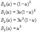
The Bi(u) are the Bézier basis functions, which are cubic Bernstein polynomials. The Bernstein polynomials used for a cubic Bézier curve take this form:

Here are the same equations expanded out:

These basis functions indicate the proportion that each control point influences the curve. As you can see, each basis function is a cubic. They are also symmetrical (shown in Figure 1), and add up to one.

Bézier curves travel through their beginning and ending control points, but the middle control points only influence the curve, and aren't directly on the curve.

Bicubic Bézier Surfaces

A bicubic Bézier surface is a parametric surface (u,v = [0,1], [0,1]) defined by its sixteen control points which lie in a four-by-four grid, pij. The common form for representing this surface is:

The functions Bi(u) and Bj(v) are the same Bernstein polynomials which were shown for the Bézier curve.

The edges of Bézier surfaces are each Bézier curves defined by the control points along that edge. The only control points that lie on the surface are the corner control points. In order to generate the surface, we need to compute points from the surface representation given above, defined by the sixteen control points. This tessellation can be done in a variety of ways. Let's look at three of them and examine the cost of creating a 9x9 grid of vertices on the surface.

Tessellation by Direct Evaluation

The most obvious way to slice a Bézier surface into polygons is by directly calculating the double-sum equation on a regular grid. Directly calculating a point on the surface costs 51 adds and 116 multiplies when done in a fairly efficient manner. Since we can calculate all 81 points iteratively, some of these computations can be amortized across the rows or down the columns of the grid. Without doing too much extra programming it is possible to compute all 81 vertices using direct evaluation at a cost of 3978 adds and 8586 multiplies.

Tessellation by De Casteljau's Algorithm

Another way to tessellate a Bézier surface is through the use of De Casteljau's algorithm. De Casteljau's algorithm shows how a Bézier curve can be calculated by using simple linear interpolation between control points. Calculating points on a Bézier curve via De Casteljau's algorithm is similar to direct evaluation of points on the curve. But we can construct an algorithm to generate surface points by splitting surfaces from De Casteljau's algorithm, and that should increase the speed of surface tessellation.

Take a look at Figure 2 for an illustration of how De Casteljau's algorithm works. Start with lines connecting each pair of the Bézier curve's adjacent control points (P0 to P1, P1 to P2, P2 to P3). The parameter t ([0,1]) represents a distance along each of these lines, where 0 is the beginning of the line, and 1 is the end. At t along each line put a mark. Connect adjacent marks (call them P01, P12, P23) with lines, and again make a mark at t on each of those lines. Connect these two marks (P02, P13) and drop a point at t (P03) on this line. That point lies on the Bézier curve. If you step the parameter t from 0 to 1, you will produce the entire curve.

This is a pretty simple algorithm and it can easily be used to split curves in half if you set t=0.5. This will generate two smaller Bézier curves with their own sets of control points. The control points of the subcurves are actually the intermediate marks we made during the split process.

And we can use this curve-splitting technique to split our Bézier surface into subsurfaces! At each stage we start with a bicubic Bézier surface that has four rows of four control points each. Split all four rows of control points in half using De Casteljau's algorithm at each row, and we then have two separate Bézier surfaces, each with their own sets of control points. Since these are subsurfaces of the original surface, the corner control points of the subsurfaces are points that lie on the original Bézier surface.

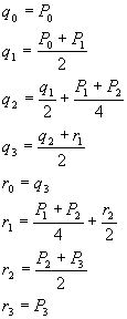
To compute the control points of the subcurves we can generate equations directly from the description above. Here are the equations that will generate the new sets of control points qi and ri:

The point q3 (also known as r0) is the curve splitting point. This set of equations will generate two subcurves with their control points, at a cost of 18 adds and 18 multiplies. (6 adds and 6 multiplies for each of x, y, and z.)

A surface split takes four curve splits so it costs four times that, or 72 adds and 72 multiplies. We need to do 51 surface splits (optimized from 63) to tessellate our entire surface, so the total comes to 3672 adds and 3672 multiplies.

Although this algorithm is indeed cheaper than direct evaluation, a drawback is how much extra data we have to keep around. Keeping track of all the control points necessary for each subsurface is a lot of data. For computation of Bézier surfaces in a limited memory space (the Nintendo64 RSP DMEM is only 4KB) this may be too much stuff to keep around. Let's see if we can find something better.

Tessellation by Central Differencing

A third way of generating points on a Bézier surface is through the use of central differencing [CLAR79]. In this approach we look at taking advantage of the Bézier curves on the edges of the surface, by splitting the edge curves and then splitting across the surface repeatedly to subdivide the surface. Using central differencing we can very quickly compute the midpoint of a Bézier curve, so this should speed up our tessellation even further. Let's derive the algorithm for surface splitting.

We start with the Taylor series expansion, which represents the value of a function Q near a point u.

In this equation, Qi(u) is the i-th derivative of Q(u).

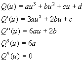
The functions that describe a Bézier curve are cubic. So we know right away that the derivatives will be of the form:

Since the fourth and higher derivatives of the cubic equation are zero, the Taylor expansion only needs to go out to the third derivative. The new form of the above equation looks like this:

If we wanted to look at points just behind u, in the negative du direction, we could work with this expression:

Let's add these two equations together to see what we can derive using points in front of and behind Q(u). Adding the equations together we receive this:

This equation is beginning to look useful. Let's simplify it to solve for Q(u):

Now imagine that we're trying to split a Bézier curve in half. If u ranges from 0 to 1, we want to find the value of the curve at u=0.5. We can also use du=0.5, to represent the entire curve. Note that these values are only valid at the first curve subdivision step for the surface. This equation simplifies even further, down to:

This shows us that the value at the midpoint of the curve, Q(0.5), is simply the average of the endpoints of the curve, minus a fraction of the second derivative at the midpoint! That's 6 adds and 6 multiplies to compute the midpoint assuming that we have the values Q(0), Q(1), and Q''(0.5).

How do we get Q''(0.5)? Let's start with the grid of 16 control points that represents the surface. Earlier I stated that the corner control points are on the Bézier surface, and that each edge is a Bézier curve. So the first step to take is splitting each edge of the surface to generate midpoints for the edge curves. We have the Q(0) and Q(1) values for each edge (the above equation works equally well in either parameter direction, u or v), but no second derivatives.

If we go through the derivation above with Q(u) replaced by Q''(u), we get a formula that helps:

Since the fourth derivative of the cubic equation is zero, the equation has reduced nicely to the form above. At the first subdivision step, this equation reduces to:

It doesn't get much easier than that. Just the average of the second derivative at the curve's endpoints! That makes sense, since Q''(u) is a linear function. But wait, we still don't have Q''(0) or Q''(1). Let's derive those.

Deriving the Second Partial Derivatives. We're working in a biparametric space. Both u and v vary across the Bézier surface. All the curve splitting we'll be doing will be along curves where one of these parameters is held constant. So the equation we need to derive is for the second derivative in the direction of the varied parameter. For curves that vary in u, what we need is the second partial derivative of u for the surface along this curve. Likewise for v-curves.

Starting with the parametric equation for the Bézier curve expanded from the sum form, we can easily compute the second derivative for the curve.

Now we have equations that we can use at the corner points of the surface to generate the second partial derivatives for both u and v. The points in the equations will correspond to the points along each edge of the surface, in the appropriate parameter direction. As we split the curves, we can average the second partials at the endpoints (as shown above) so that successive subcurves will have appropriate values for future curve splits.

This leaves one last issue. As we split the surface, we will frequently split a u-curve, take the midpoint, and use it as an endpoint for a curve to be split in v. The second partial in v is cubic across a u-curve, so we need a way to generate both second partials at each split. A previous equation that we derived can be adapted for this purpose:

This shows that we can compute the second partial derivative in v on a u-curve if we know the value of Quuvv. A similar equation shows that we can use Quuvv for v-curves as well.

Quuvv is guaranteed to be linear across the curve, so we can average the endpoints again to receive the value at the midpoint:

So now we just need the value of Quuvv at the surface corner points to start things off. This time we have to do the derivation from the original double-sum equation.

We can take the second derivative of each of the Bernstein polynomials, to plug into the above equation:

To compute Quuvv at any corner point, just plug u and v into these equations and perform the double summation.

Central Differencing Performance Analysis. We've done a lot of work here so let's review. At the initialization stage we need to compute the values Quu(u,v), Qvv(u,v) and Quuvv(u,v) at each corner point. Here are examples of what these equations look like at the corner point (u,v)=(0,0).

Performing these computations on each corner point results in a total cost of 120 adds and 180 multiplies. A pretty hefty initialization cost, to be sure!

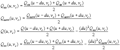
However, each curve subdivision after initialization generates one surface point and costs fairly little. These computations need to be performed at each curve split (these equations are for u-curves, but the v-curve equations are similar):

These curve splits cost 18 adds and 30 multiplies each.

We need to perform 77 curve splits in order to produce a total of 81 surface points. The total cost to do this, including initialization, is 1506 adds and 2490 multiplies. As you might guess, a lot of the computations are redundant and it is quite easy to optimize the algorithm further, to 1506 adds and 1488 multiplies.

Conclusion

Through the use of some crafty mathematical techniques, we've reduced the cost of computing a 9x9 grid of vertices on a bicubic Bézier surface from 3978 adds and 8586 multiplies, to 1506 adds and 1488 multiplies. This is much more reasonable!

The goal of this mathematical exercise was to find an algorithm for computing bicubic Bézier surfaces that would allow their use in real-time games. At the same time I wanted to find an algorithm that could be optimized for a vector processor, and for which the data would fit in the 4KB of the Nintendo64's RSP co-processor. The central differencing algorithm fits all these requirements. The curve-splitting stage of the central differencing algorithm is highly vectorizable, and the data does indeed fit in 4KB, unlike the data necessary when using De Casteljau's algorithm to split surfaces.

Further References

Sharp, Brian. "Implementing Curved Surface Geometry" (June 1999) and "Optimizing Curved Surface Geometry" (July 1999). Game Developer magazine.

Watt, Alan and Watt, Mark. Advanced Animation and Rendering Techniques: Theory and Practice. New York: ACM Press, 1992.

Clark, J.H., "A Fast Scan-Line Algorithm for Rendering Parametric Surfaces," Computer Graphics Vol 13 No.2: pp. 289-99.

If you're a Nintendo 64 developer, you can find the Bézier surface microcode that implements central differencing at Nintendo's developer web site at https://www.warioworld.com.